CFD Effectiveness = Quality x Acceptance
where,
Quality – Fidelity of Data
Acceptance – Timeliness of Data
CFD should essentially meet 3 requirements:
I. Rapid Turnaround.
II. Reliable Accuracy.
III. Affordable Cost.
A typical design process includes:
i. Pre-conceptual
ii. Conceptual
iii. Preliminary
iv. Critical
v. Production

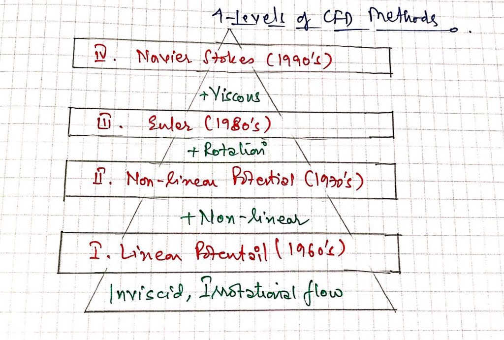
I. Linear Potential Methods
- Solve 1st order PDE
- Based on Prandtl-Glauert /Laplace equation.
- Green’s Theorem
- Surface Discretization
- Vortex-Lattice Methods (VORLAX code). Mean surface representation of geometry & vortex filaments as singularities.
- Panel Methods (Actual surface geometry discretized)
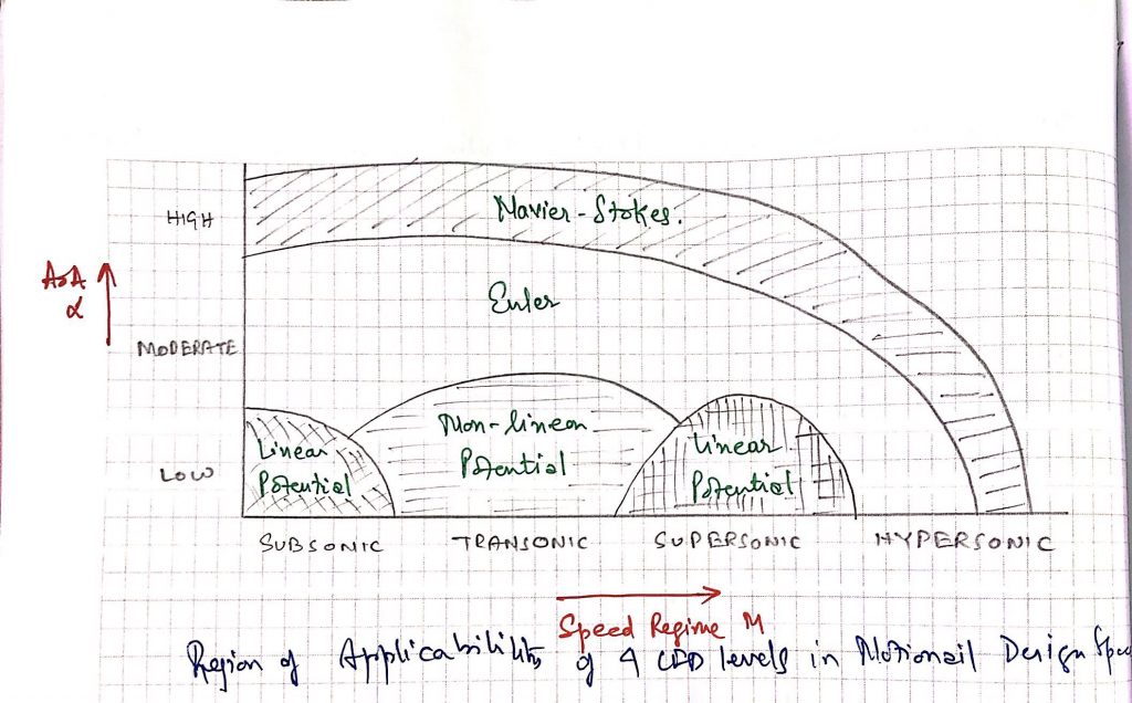
- Purely Subsonic & Supersonic flows.
- Good estimate of F & M and distributed air loads for steady-level flight.
- 1960’s, established 1980’s.
II. Non-Linear Potential Methods
- Solver 2nd order PDE
- Based on Transonic Small Perturbation (TSP) or Full Potential Equation ( FPE).
- Benefit of modelling transonic flows with Shocks.
- Need to solve non-linear PDE’s.
III. Euler Methods
- Highest level of Inviscid approximations.
- Subsonic to Hypersonic regimes.
- Captures Potential flow regimes (Wake sheds from wing & leading edges)
- Solving atleast 4 and generally 5 coupled 1st order PDE’s instead of one 2nd order PDE.
- 1980’s : Structured Grid Generation, Patched Multiblock, Overset Mesh
- Mid 1980’s : Unstructured grid generation.
- Convergence acceleration techniques- i) Local time-stepping, ii) Multi-Grid (FMG)
- Explicit and Implicit time-marching schemes.
- Time dependent equations
- Codes didnot provide Total Drag (incl. Skin Friction) and thus N-S codes were pursued in parallel.
IV. Navier-Stokes Method
- Same equation except the diffusion terms in N-S solver
- Elimination of the diffusion term converts the N-S equations to Euler equations as they both share some convective terms.
- RANS- Turbulence Model – Simple algebraic model to sophisticated Reynolds’ Stress model.
